PolitiFact - 10+ Years of Fact Checking
James Midkiff
This is the R code I used to generate the analysis. Feel free to use portions of it for your own non-commercial work, but if you use all of the code then please attribute it to me.
# Here is the R code that generated this entire analysis feel free to copy sections of it but if you're re-running the entire thing, please attribute it to me.
# Code author:  James Midkiff

knitr::opts_chunk$set(echo = TRUE)
library(tidyverse)
library(lubridate)
library(stringr) #I love this package and Regular Expressions
library(tidytext)
library(scales)
library(RColorBrewer)
library(rvest) #Scraping package - highly recommend following the tutorial and using a CSS Selector
library(forcats)
library(knitr) #For RMarkdown
library(BSDA) #Used for Z-Test only
rm(list = ls()) #Careful, this will wipe out your environment
# Scrape#########
# I recommend that you minimize everything (Alt + O) and then uncover it section by section as you go through it since it's a lot of code. I'm going to clear the envirnoment first and then save everything as an image that I can then use for the other page without code.
webpage <- read_html("http://www.politifact.com/truth-o-meter/statements/")
no_pages <- html_text(html_nodes(webpage, '.step-links__current'))
no_pages <- as.integer(
str_extract(no_pages, "\\d{3,4}(?=\n)")) #A quick scrape to determine how many pages there are on PolitiFact's website
name <- vector("list", length = no_pages)
source <- vector("list", length = no_pages)
date <- vector("list", length = no_pages)
picture_rating <- vector("list", length = no_pages)
statement_text <- vector("list", length = no_pages)
explanation_text <- vector("list", length = no_pages)
rating <- vector("list", length = no_pages)
#This is the for loop for scraping all of PolitiFact's statements.
for (i in seq_along(1:length(name))) {
webpage <- read_html(
str_c("http://www.politifact.com/truth-o-meter/statements/?page=", i))
politifact_scrape <- function(x) {
as_tibble(
html_text(
html_nodes(webpage, x)))
}
name[[i]] <- politifact_scrape('.statement__source a')
source[[i]] <- politifact_scrape('.statement__edition a')
date[[i]] <- politifact_scrape('.article__meta')
statement_text[[i]] <- politifact_scrape('.statement__text')
explanation_text[[i]] <- politifact_scrape('.quote')
#Take the image, use the alt-text to find the rating
attributes <- html_attrs(
html_nodes(webpage, '.meter img'))
for (j in seq_along(attributes)) {
rating[[i]][[j]] <- attributes[[j]][[2]]
}
rating[[i]] <- as_tibble(rating[[i]])
Sys.sleep(time = 3) # Do a 3 second pause before running the loop again
# This should take approximately 4 seconds (1 second of 'for loop' run time
# plus a 3 second mandatory wait) times 700-some pages divided by 60 seconds per
# minute = ~50 minutes
}
options(max.print = 50)
#Setting the appropriate length for the final dataset
(length_each_page <- length(name[[1]][[1]]))
(length_last_page <- length(name[[no_pages]][[1]]))
#Subtract one b/c last page isn't complete
(total_length <- (no_pages - 1) * length_each_page + length_last_page)
politifact <- tibble(yup = 1:total_length)
combining_function <- function(df, x) {
tibblez <- do.call("rbind", x)
var_name <- substitute(x)
df %>%
bind_cols(tibblez) %>%
rename(!!var_name := value) %>%
select(-yup)
}
(combined_name <- combining_function(politifact, name))
(combined_source <- combining_function(politifact, source))
(combined_date <- combining_function(politifact, date))
(combined_statement_text <- combining_function(politifact, statement_text))
(combined_explanation_text <- combining_function(politifact, explanation_text))
(combined_rating <- combining_function(politifact, rating))
#This below is the original dataset
politifact_orig <- bind_cols(combined_name, combined_source, combined_date,
combined_statement_text, combined_explanation_text,
combined_rating)
politifact_orig <-
politifact_orig %>%
mutate(name = str_replace_all(name, "^\\s+", ""),
source = str_replace_all(source, "^.{2}", ""),
rating = str_trim(rating),
date = mdy(
str_replace_all(date, "^.+, (?=\\D)", "")),
rating = fct_relevel(as_factor(rating), c("Pants on Fire!", "False",
"Mostly False", "Half-True",
"Mostly True", "True",
"Full Flop", "Half Flip",
"No Flip")))
(rating_type <- tibble(
rating = c("Pants on Fire!", "False", "Mostly False", "Half-True",
"Mostly True", "True", "Full Flop", "Half Flip", "No Flip"),
Type = c(rep("Truth-O-Meter", 6), rep("Flip-O-Meter", 3)))) #This is a way of setting up which statements belong to the Truth-O-Meter vs the Flip-O-Meter
rating_type <- rating_type %>%
mutate(rating = fct_relevel(
as_factor(rating), levels(politifact_orig$rating)))
politifact_orig <- left_join(politifact_orig, rating_type, by = "rating")
politifact_orig <- politifact_orig %>%
mutate(website = if_else(str_detect(name, "\\.com|\\.net|\\.gov|\\.org|\\.edu|\\.us|\\.site$"),
TRUE, FALSE),
website = if_else(str_detect(name, regex("blog|facebook|(e|e-)mail|image|tweets|online|infowars", ignore_case = TRUE)), #Flag all of this as a website
TRUE, website),
source = str_replace_all(source, "^\\s|\\s$", ""), #Clean leading/trailing spaces
politifact_location = if_else(str_detect(source, "National|PunditFact|NBC|Global"),
"Not State", "State")) #State edition or not
#I will generally be working with this dataset, which is only truth-o-meter statements
politifact <- politifact_orig %>%
filter(Type == "Truth-O-Meter")This analysis was conducted at 2018-01-09 16:52:56 and only captures statement ratings PolitiFact published before that time. This project should auto-update each time that I re-run the R script.
1. Background
#This generates the page number for people to look for to verify that there are not November 2008 ratings. If PolitiFact ever puts them up, I will take this section and the footnote out.
page_series <- tibble(contains = str_detect(date, "December 1st, 2008"),
                      page_no = 1:length(date))
page_series <- page_series %>%
  filter(contains == TRUE)

see_this_nov_2008 <- max(page_series$page_no)
According to its website, PolitiFact is a “fact-checking website that rates the accuracy of claims by elected officials and others who speak up in American politics.” The goal of this project is to analyze all of the ratings that PolitiFact has issued since it began in 2007 and to look for trends and other curiosities in the data. Besides strengthening my data analysis and mark-up skills, my motivations for this project have been my admiration of PolitiFact’s non-partisan fact-checking and my own simple curiosity.
#Number of total ratings by PolitiFact. This shows up in the paragraph below. 'V' is my attempt at saying a number that I will use as part of inline code in the narrative.
V_Total_Ratings <- comma_format()(as.integer
                                  (politifact_orig %>%
                                      summarise(Total_Ratings = n())))
The most recent statements evaluated by PolitiFact appear at this page, (http://www.politifact.com/truth-o-meter/statements/). As of the date and time I ran this code, PolitiFact has evaluated a total of 14,181 ratings. [^1]
1.1 Truth-O-Meter vs. Flip-O-Meter
On its site, PolitiFact evaluates statements using either its Truth-O-Meter or its Flip-O-Meter system. In short, the Truth-O-Meter is used to evaluate statements for their accuracy (did the speaker say the truth, a falsehood, or something in between?), while the Flip-O-Meter is used to evaluate an official’s consistency on an issue (did they maintain their position, or partly/completely change their stance on a topic?).
#Number and Proportions for total statements in Truth-O-Meter and Flip-O-Meter
temp <- politifact_orig %>%
  group_by(Type) %>%
  summarise(Subtotal = n()) %>%
  mutate(Proportion = round((Subtotal / sum(Subtotal)) * 100, 1),
         Subtotal = comma_format()(Subtotal))

V_Flip_O_Meter_n <- temp %>%
  filter(Type == "Flip-O-Meter") %>%
  select(Subtotal)
V_Flip_O_Meter_prop <- temp %>%
  filter(Type == "Flip-O-Meter") %>%
  select(Proportion)

V_Truth_O_Meter_n <- temp %>%
  filter(Type == "Truth-O-Meter") %>%
  select(Subtotal)
V_Truth_O_Meter_prop <- temp %>%
  filter(Type == "Truth-O-Meter") %>%
  select(Proportion)
From here on, my analysis will focus only on those statements evaluated by the Truth-O-Meter since they are much more numerous. There are 13,950 (98.4%) Truth-O-Meter Ratings and 231 (1.6%) Flip-O-Meter Ratings.
PolitiFact assigns statements one of six possible ratings to Truth-O-Meter Ratings:
TRUE - The statement is accurate and there’s nothing significant missing.
MOSTLY TRUE - The statement is accurate but needs clarification or additional information.
HALF TRUE - The statement is partially accurate but leaves out important details or takes things out of context.
MOSTLY FALSE - The statement contains an element of truth but ignores critical facts that would give a different impression.
FALSE - The statement is not accurate.
PANTS ON FIRE - The statement is not accurate and makes a ridiculous claim.
For more information on how PolitiFact selects and evaluates statements, see here.
2. Truth-O-Meter Summary Statistics
#Truth-o-Meter Summary Stats
truth_o_meter_ratings <- politifact %>%
  rename(Rating = rating) %>%
  group_by(Rating) %>%
  summarise(Total_Ratings = n()) %>%
  mutate(Proportion = Total_Ratings / sum(Total_Ratings))
#I used ColorPick Eyedropper to select the colors straight from the PolitiFact graphics
truth_o_meter_colors <- c("#E40602", "#E71F28", "#EE9022", "#FFD503", "#C3D52D", "#71BF44")
ggplot(truth_o_meter_ratings, aes(x = Rating, y = Proportion, fill = Rating)) +
labs(title = "PolitiFact Truth-O-Meter Ratings Since 2017") +
geom_col(color = "black", size = 1) +
geom_label(label = comma_format()(truth_o_meter_ratings$Total_Ratings)) +
scale_fill_manual(values = truth_o_meter_colors) +
scale_y_continuous(labels = percent) +
theme(legend.position = "none") 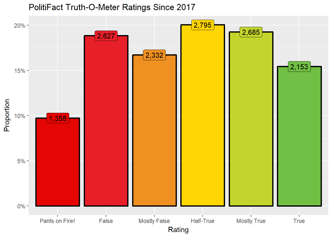
#Truthhoods vs. Falsehoods numbers and percentages
V_truthful <- truth_o_meter_ratings %>%
  filter(Rating == c("Mostly True", "True")) %>%
  summarise(Proportion = sum(Proportion)) %>%
  mutate(Proportion = percent_format()(Proportion))
V_truthful <- as.vector(V_truthful$Proportion)

V_false <- truth_o_meter_ratings %>%
  filter(Rating == c("Pants on Fire!", "False", "Mostly False")) %>%
  summarise(Proportion = sum(Proportion)) %>%
  mutate(Proportion = percent_format()(Proportion))
V_false <- as.vector(V_false$Proportion)

V_half_true <- truth_o_meter_ratings %>%
  mutate(Proportion = percent_format()(Proportion)) %>%
  filter(Rating == "Half-True")
V_half_true <- as.vector(V_half_true$Proportion)
If we consider “truths” to be those statements PolitiFact rated as Mostly True or True and “falsehoods” to be those rated as Pants on Fire!, False, or Mostly False, then 34.7% of the total statements rated were truths, 45.3% of the total statements rated were falsehoods, and the remaining 20.0% statements were Half-True . As such, PolitiFact has rated more statements as falsehoods than as truths; whether this represents a selection bias on PolitiFact’s part or the nature of American political rhetoric is something not possible to say with this data alone.
2.1 Rating Issuer
#The locations/editions of PolitiFact summary stats
locations <- politifact %>%
  group_by(source) %>%
  mutate(Founded = min(year(date))) %>%
  group_by(source, Founded, politifact_location) %>%
  summarise(Total_Ratings = n()) %>%
  arrange(-Total_Ratings) %>%
  ungroup() %>%
  mutate(`Percentage of Total Ratings` = percent_format()(Total_Ratings / sum(Total_Ratings))) %>%
  rename(Issuer = source, Type = politifact_location)

locations <- locations %>%
  add_column(Rank = 1:nrow(locations)) %>%
  select(Rank, everything())

#Merging in the electoral votes for each state, from https://state.1keydata.com/state-electoral-votes.php
#don't forget Washington DC
electoral_votes <- tribble(
~US_State,  ~`Electoral Votes`,
"Alabama", 9,
"Montana", 3,
"Alaska", 3,
"Nebraska", 5,
"Arizona", 11,
"Nevada", 6,
"Arkansas", 6,
"New Hampshire", 4,
"California", 55,
"New Jersey", 14,
"Colorado", 9,
"New Mexico", 5,
"Connecticut", 7,
"New York", 29,
"Delaware", 3,
"North Carolina", 15,
"Florida", 29,
"North Dakota", 3,
"Georgia", 16,
"Ohio", 18,
"Hawaii", 4,
"Oklahoma", 7,
"Idaho", 4,
"Oregon", 7,
"Illinois", 20,
"Pennsylvania", 20,
"Indiana", 11,
"Rhode Island", 4,
"Iowa", 6,
"South Carolina", 9,
"Kansas", 6,
"South Dakota", 3,
"Kentucky", 8,
"Tennessee", 11,
"Louisiana", 8,
"Texas", 38,
"Maine", 4,
"Utah", 6,
"Maryland", 10,
"Vermont", 3,
"Massachusetts", 11,
"Virginia", 13,
"Michigan", 16,
"Washington", 12,
"Minnesota", 10,
"West Virginia", 5,
"Mississippi", 6,
"Wisconsin", 10,
"Missouri", 10,
"Wyoming", 3,
"Washington D.C.", 3)

locations <-
  locations %>%
  separate(Issuer, c("A", "State"), sep = 11, remove = FALSE)

locations <- left_join(locations, electoral_votes, by = c("State" = "US_State"))%>%
  select(-A, -State) %>%
  mutate(Total_Ratings = comma_format()(Total_Ratings)) %>%
  rename(`Total Ratings` = Total_Ratings) %>%
  select(everything(), `Electoral Votes`)
#Most important Editions
top_x_issuers <- locations %>%
filter(`Percentage of Total Ratings` >= 1) %>% #Only takes those with individually more than 1% of the ratings
mutate(Cumulative_Sum = percent_format()(cumsum(
as.numeric(
str_replace_all(`Percentage of Total Ratings`, "[[:punct:]]", "")) / 1000)))
values <- tibble(rating = levels(politifact$rating)[1:6], value = seq(-3, 2, 1)) %>%
mutate(rating = as_factor(rating),
rating = fct_relevel(rating, levels(politifact$rating)))
locations_rating <- politifact %>%
group_by(source, rating) %>%
summarise(Total_Ratings = n())
locations_rating <- left_join(locations_rating, values, by = "rating") %>%
mutate(score = Total_Ratings * value) %>%
summarise(Score = round((sum(score) / sum(Total_Ratings)), 3))
one_percent_issuers <- left_join(top_x_issuers, locations_rating, by = c("Issuer" = "source")) %>%
mutate(Issuer = factor(Issuer),
Issuer = fct_reorder(Issuer, Score)) %>%
arrange(Score)
one_percent_issuers <- one_percent_issuers %>%
mutate(cut = cut_interval(one_percent_issuers$Score, 12)) PolitiFact is made up of various “Editions” that focus on different sources for the statements that they will rate. There are a total of 25 editions, which I have grouped into two main categories: “State” Editions that focus on statements made by officials or people in a certain U.S. state (21 such editions) and “Non-State” Editions that do not focus on a a single state (the remaining 4 editions). These 21 State Editions cover states with a total of 345 electoral votes, equal to 64.1% of the total electoral votes available for presidential elections.
As we see from this table, PolitiFact National was the source for over one-third of the total statements evaluated. This is likely due in part to the fact that it was the earliest edition founded. The other “Not State” editions include PunditFact, which evaluates statements made by political pundits, PolitiFact Global News Service, which evaluates statements made about Health and Development, and PolitiFact NBC, which is a partnership between PolitiFact and NBC.
#Kable is Rmarkdown's way of making a table look good
kable(locations, align = c("l", "l", "r", "r", "r", "r", "r"),
caption = "The Various PolitiFact Editions")| Rank | Issuer | Founded | Type | Total Ratings | Percentage of Total Ratings | Electoral Votes |
|---|---|---|---|---|---|---|
| 1 | PolitiFact National | 2007 | Not State | 4,662 | 33.4% | NA |
| 2 | PolitiFact Florida | 2009 | State | 1,435 | 10.3% | 29 |
| 3 | PolitiFact Texas | 2010 | State | 1,354 | 9.7% | 38 |
| 4 | PolitiFact Wisconsin | 2010 | State | 1,259 | 9.0% | 10 |
| 5 | PunditFact | 2013 | Not State | 948 | 6.8% | NA |
| 6 | PolitiFact Georgia | 2010 | State | 862 | 6.2% | 16 |
| 7 | PolitiFact Ohio | 2010 | State | 591 | 4.2% | 18 |
| 8 | PolitiFact Rhode Island | 2010 | State | 544 | 3.9% | 4 |
| 9 | PolitiFact Virginia | 2010 | State | 537 | 3.8% | 13 |
| 10 | PolitiFact New Jersey | 2011 | State | 395 | 2.8% | 14 |
| 11 | PolitiFact Oregon | 2010 | State | 390 | 2.8% | 7 |
| 12 | PolitiFact New Hampshire | 2011 | State | 153 | 1.1% | 4 |
| 13 | PolitiFact California | 2015 | State | 121 | 0.9% | 55 |
| 14 | PolitiFact Global News Service | 2016 | Not State | 91 | 0.7% | NA |
| 15 | PolitiFact Missouri | 2015 | State | 90 | 0.6% | 10 |
| 16 | PolitiFact New York | 2016 | State | 88 | 0.6% | 29 |
| 17 | PolitiFact North Carolina | 2016 | State | 88 | 0.6% | 15 |
| 18 | PolitiFact Pennsylvania | 2016 | State | 80 | 0.6% | 20 |
| 19 | PolitiFact Tennessee | 2012 | State | 76 | 0.5% | 11 |
| 20 | PolitiFact Illinois | 2016 | State | 63 | 0.5% | 20 |
| 21 | PolitiFact Nevada | 2016 | State | 41 | 0.3% | 6 |
| 22 | PolitiFact Arizona | 2016 | State | 38 | 0.3% | 11 |
| 23 | PolitiFact Colorado | 2016 | State | 29 | 0.2% | 9 |
| 24 | PolitiFact Iowa | 2015 | State | 12 | 0.1% | 6 |
| 25 | PolitiFact NBC | 2016 | Not State | 3 | 0.0% | NA |
Given that only a subset of all of the PolitiFact Editions are responsible for the vast majority of the statement ratings, I am going to focus on those Editions which individually were responsible for more than 1% of the Truth-O-Meter ratings. These top 12 PolitiFact Editions were cumulatively responsible for 94.0% of the total statements rated.
Looking at the most important PolitiFact Editions, I have set up a metric to measure the average truthfulness of the statements that they have rated. Any statement that is rated as True, I have assigned a Truthfulness Score of +2. Likewise, any statement that PolitiFact has rated False, I have assigned a Truthfulness value of -2. Mostly True, Half-True, and Mostly False statements thus correspond to scores of +1, 0, and -1 respectively. Pants on Fire! claims are “False” statements that are especially ridiculous, so I have given them a Truthfulness Score of -3 (see Table below).
#I came up with this metric myself
kable(values %>%
        rename(`Statement Rating` = rating, `Truthfulness Score` = value) %>%
        arrange(desc(`Truthfulness Score`)),
caption = "Truthfulness Score per Statement Rating")| Statement Rating | Truthfulness Score |
|---|---|
| True | 2 |
| Mostly True | 1 |
| Half-True | 0 |
| Mostly False | -1 |
| False | -2 |
| Pants on Fire! | -3 |
Using then the top 12 PolitiFact Editions, I have generated a Mean Truthfulness Score for all of the statements PolitiFact has examined. This number takes the total number of statements by rating (e.g. True, Mostly True, etc.), the Truthfulness Score I have assigned each rating, and then divides the sum of those Truthfulness values by the total number of ratings that each Edition has made. In other words, this metric says “What is the average truthfulness of a statement evaluated by each PolitiFact Edition?”.
As we see from the graph below, PunditFact has the lowest average Truthfulness score at -1.148, which means that the average statement that PunditFact rates is Mostly False. Rounding out the top three, PolitiFact Wisconsin and PolitiFact National were the next Editions with the lowest average Truthfulness Scores. On the other end of the spectrum PolitiFact Georgia and PolitiFact Ohio were the only Editions who had a positive truthfulness rating, meaning that the average statement they rated was at least Half-True.
ggplot(one_percent_issuers, aes(x = Issuer, y = Score, fill = cut)) +
  labs(x = "PolitiFact Edition (i.e. who rated the statement?)",
       y = "Average Truthfulness Rating",
       title = "Mean Truthfulness Score by PolitiFact Edition") +
  geom_col(color = "black", size = 1) +
  geom_label(label = one_percent_issuers$Score) +
  scale_x_discrete(labels = c(
    "PolitiFact Wisconsin" = "PolitiFact\n Wisconsin",
    "PolitiFact National" = "PolitiFact\n National",
    "PolitiFact Rhode Island" = "PolitiFact\n Rhode Island",
    "PolitiFact New Hampshire" = "PolitiFact\n New Hampshire",
    "PolitiFact Virginia" = "PolitiFact\n Virginia",
    "PolitiFact Texas" = "PolitiFact\n Texas",
    "PolitiFact Florida" = "PolitiFact\n Florida",
    "PolitiFact Oregon" = "PolitiFact\n Oregon",
    "PolitiFact New Jersey" = "PolitiFact\n New Jersey",
    "PolitiFact Ohio" = "PolitiFact\n Ohio",
    "PolitiFact Georgia" = "PolitiFact\n Georgia")) +
  scale_fill_manual(values = c("#E40602", "#D0240D", "#BD4318", "#AA6223", "#97812E", "#84A039", "#71BF44")) +
  theme(legend.position = "none")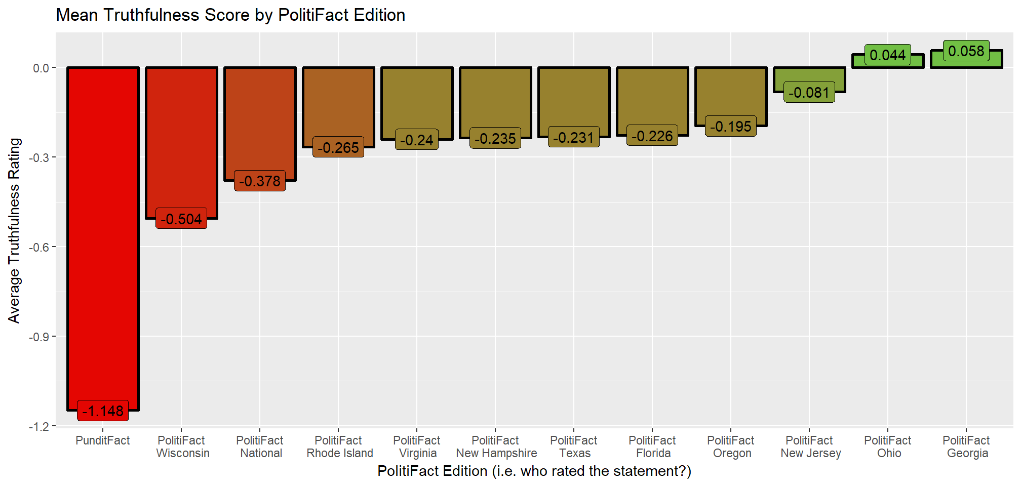
2.2 Ratings Over Time
Given that PolitiFact provides the date that it has rated each statement, it may be interesting to explore if the relative truthfulness of the statements rated has changed over time. Since mid-2010, PolitiFact has generally issued about 3-4 statement ratings per day. In the below graph, I have taken the Mean Truthfulness Score for all of the statements that PolitiFact has evaluated each month (excluding months where PolitiFact rated fewer than 30 statements) and a smooth line to estimate the average Mean Truthfulness Score over time.
Some interesting trends present themselves.
avg_score_all <- politifact %>%
  group_by(rating) %>%
  summarise(n = n())

avg_score_all <- left_join(avg_score_all, values, by = c("rating" = "rating")) %>%
  mutate(score = value * n) %>%
summarise(avg_value = sum(score) / sum(n)) #The average score for PolitiFact Truth-O-Meter's history- The Mean Truthfulness Score for each month is generally negative (the overall rating for all statements PolitiFact has rated was -0.33). There were only two occasions where the Mean Truthfulness Score was notably positive for a few months in a row: September and October of 2007 (early in PolitiFact’s rating history) and around December 2012 / January 2013. To a smaller extent, this same positive blip also occurred in December 2014 / January 2015. Maybe the PolitiFact staff around the holiday season join in the spirit of giving by becoming more generous with their ratings?
- I had thought that the presidential campaign season, which for the sake of argument I have set as one-year prior to the presidential election, would have seen several months with particularly low Mean Truthfulness Scores. My thinking was that close to the presidential election, politicians would be less truthful in order to capture undecided voters at the last minute. At least from this graph, these factors appear to be uncorrelated though that may be due to the fact that there are not many presidential candidates per election and the number of them decreases as the election date approaches which in turn generates fewer statements for PolitiFact to rate.
year_score_all_pre_na <- politifact %>%
  mutate(revised_date = date)
day(year_score_all_pre_na$revised_date) <- 1 #Setting all the days to day = 1 so that way they're grouped by month

year_score_all_pre_na <- year_score_all_pre_na %>%
  group_by(revised_date, rating) %>%
  summarise(n = n())

year_score_all_pre_na <- left_join(year_score_all_pre_na, values, by = c("rating" = "rating")) %>%
  ungroup() %>%
  mutate(Score = n * value) %>%
  group_by(revised_date) %>%
  summarise(Score = round((sum(Score) / sum(n)), 3),
            Total_Ratings = sum(n))

year_score_all <- year_score_all_pre_na %>%
  mutate(Score = ifelse(Total_Ratings < 30, NA, Score)) %>% #Only dealing with those with more than 30+ ratings a month
  separate(revised_date, into = c("Year", "Month", "Junk"), remove = FALSE) %>%
  mutate(Month = str_replace_all(Month, c("01" = "Jan", "02" = "Feb", "03" = "Mar",
                                          "04" = "Apr", "05" = "May", "06" = "Jun",
                                          "07" = "Jul", "08" = "Aug", "09" = "Sep",
                                          "10" = "Oct", "11" = "Nov", "12" = "Dec"))) %>%
  unite(Label, Month, Year, sep = " ") %>%
  select(-Junk)
lowest_score_ever <- min(year_score_all$Score, na.rm = TRUE)
worst_month <- year_score_all %>%
filter(Score == lowest_score_ever) %>%
mutate(Label = str_replace_all(Label, c("Jan" = "January", "Feb" = "February", "Mar" = "March",
"Apr" = "April", "May" = "May", "Jun" = "June", "Jul" = "July",
"Aug" = "August","Sep" = "September", "Oct" = "October",
"Nov" = "November", "Dec" = "December")))- The Mean Truthfulness Score for each month has become remarkably negative since April 2017, with the record low in December 2017 at -1.359 as you can see in the graph below. Each month since April (except October) has broken the previously low record set in August 2009. Why is this so? Some possible ideas may be:
- Increased political polarization whereby politics has gotten to the point where candidates will say anything to win
- An artefact of the post-truth era some pundits think we have entered into?
- Donald Trump and his notoriety for telling falsehoods
- Or is there some other explanation?
- Increased political polarization whereby politics has gotten to the point where candidates will say anything to win
ggplot(year_score_all %>% slice(5:nrow(year_score_all)), #Lop off the first 4 rows because they're NA
aes(x = revised_date + 15, y = Score, fill = Score)) + #Add 15 days to each month so they align better
geom_rect(xmin = ymd("2016-Nov-8") - 365, xmax = ymd("2016-Nov-8"),
ymin = -3, ymax = 2, fill = "gray75", color = "black", linetype = "dashed", size = .8) +
geom_rect(xmin = ymd("2012-Nov-6") - 365, xmax = ymd("2012-Nov-6"),
ymin = -3, ymax = 2, fill = "gray75", color = "black", linetype = "dashed", size = .8) +
geom_rect(xmin = ymd("2008-Nov-4") - 365, xmax = ymd("2008-Nov-4"),
ymin = -3, ymax = 2, fill = "gray75", color = "black", linetype = "dashed", size = .8) +
geom_col(color = "black", size = 1) +
geom_smooth(size = 1.7, color = "royalblue4", se = FALSE) +
scale_x_date(date_breaks = "1 year", date_labels = "%Y") +
scale_y_continuous(breaks = seq(-1.5, 0.5, 0.25)) +
scale_fill_continuous(low = "#E40602", high = "#71BF44") +
theme(legend.position = "none",
axis.text.x = element_text(size = 12),
axis.text.y = element_text(size = 10)) +
labs(x = "",
title = "PolitiFact Mean Truthfulness Score per Month",
subtitle = "Only months with 30 or more ratings are included. Shaded areas indicate the 12 months prior to a U.S. presidential election") +
geom_point(data = worst_month, aes(x = revised_date + 15, y = Score - .10),
size = 5, color = "black", fill = "red", shape = 24, stroke = 2,
inherit.aes = FALSE) +
geom_text(data = worst_month, aes(x = revised_date + 15, y = Score - .2),
label = "Minimum", inherit.aes = FALSE, color = "black", fontface = "bold")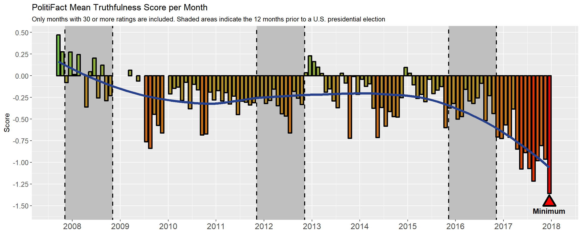 ### 2.3 Recent Ratings Seeing as how quickly PolitiFact’s monthly Mean Truthfulness Score becomes very negative after the 2016 presidenital election, I decided to separate the ratings into three mutually exclusive categories to figure out why:
- I flagged as Website any rating of a statement made by an entity ending in .com, .net, .org, .us, .edu, .site, .gov or that had the word email, facebook, blog, tweet, or image in its name.
- I flagged as Trump any rating of a statement made by Donald Trump.
- I flagged all other ratings as Other.
I took the subtotal Mean Truthfulness values for these three statement categories and divided by the total number of ratings issued each month by PolitiFact. These steps allows me to determine what each of the three categories contributed to PolitiFact’s total Mean Truthfulness Score for each month.
trump_web_other <- politifact %>%
  mutate(analysis = NA)
trump_web_other <- politifact %>%
  mutate(analysis = ifelse(website == TRUE, "Website", NA),
         analysis = ifelse(name == "Donald Trump", "Trump", analysis),
         analysis = ifelse(is.na(analysis), "Other", analysis))

trump_web_analysis <- trump_web_other %>%
  mutate(revised_date = date)
day(trump_web_analysis$revised_date) <- 1 #Setting all the days to day = 1 so that way they're grouped by month

trump_web_analysis <- trump_web_analysis %>%
  group_by(revised_date, rating, analysis) %>%
  summarise(n = n())

trump_web_analysis <- left_join(trump_web_analysis, values, by = c("rating" = "rating")) %>%
  ungroup() %>%
  mutate(Score = n * value) %>%
  group_by(revised_date, analysis) %>%
  summarise(subtotal = sum(Score),
            Subtotal_Ratings = sum(n))

trump_web_analysis <- left_join(trump_web_analysis, year_score_all_pre_na) %>%
  mutate(Sub_Score = round(subtotal / Total_Ratings, 3))
trump_web_analysis <- trump_web_analysis[c(1:4, 7, 5:6)] #Reordering columns

trump_web_analysis <- trump_web_analysis %>%
  mutate(Score = ifelse(Total_Ratings < 5, NA, Score)) %>% #Only dealing with those with more than 30+ ratings a month
  separate(revised_date, into = c("Year", "Month", "Junk"), remove = FALSE) %>%
  mutate(Month = str_replace_all(Month, c("01" = "Jan", "02" = "Feb", "03" = "Mar",
                                          "04" = "Apr", "05" = "May", "06" = "Jun",
                                          "07" = "Jul", "08" = "Aug", "09" = "Sep",
                                          "10" = "Oct", "11" = "Nov", "12" = "Dec"))) %>%
  unite(Label, Month, Year, sep = " ") %>%
  select(-Junk)

website_contribution_worst <- trump_web_analysis %>%
  filter(revised_date %in% worst_month$revised_date,
         analysis == "Website") %>%
  mutate(percentage = Sub_Score / Score)
trump_contribution_worst <- trump_web_analysis %>%
  filter(revised_date %in% worst_month$revised_date,
         analysis == "Trump") %>%
  mutate(percentage = Sub_Score / Score)
other_contribution_worst <- trump_web_analysis %>%
  filter(revised_date %in% worst_month$revised_date,
         analysis == "Other") %>%
  mutate(percentage = Sub_Score / Score)
For example, in December 2017 for all of PolitiFact there were 78 total statements rated with a Mean Truthfulness Score of -1.359. This value correlates to the average statement being at least Mostly False, and this month has the lowest Mean Truthfulness Score since PolitiFact was founded as you can again see in the graph below. Of that -1.359 Mean Truthfulness Score:
- With 15 statements rated, Websites contributed -0.5 to this month’s Mean Truthfulness Score, equal to 36.8% of it
- With 7 statements rated, Donald Trump contributed -0.115 to this month’s Mean Truthfulness Score, equal to 8.46% of it
- And the remaining 56 statements rated contributed -0.744 to this month’s Mean Truthfulness Score, equal to the remaining 54.7% of it
#When was the first website rating issued. I'm only taking the averages since that point.
first_website <- politifact %>%
  filter(website == TRUE) %>%
  filter(date == min(date))

websites_by_month <- trump_web_analysis %>%
  filter(analysis == "Website",
         revised_date >= first_website$date[[1]]) %>%
  mutate(pre_dec_2016 = ifelse(revised_date < "2016-12-01", "PRE", "POST")) %>%
  group_by(pre_dec_2016) %>%
  summarise(avg_per_month = round(sum(Subtotal_Ratings) / n(), 1),
            months = n(),
            avg_rating = round(sum(subtotal) / sum(Subtotal_Ratings), 3))
Since December 2016, ratings of statements made by websites have been the single largest contributor to the highly negative Mean Truthfulness Scores of late. This coincides with the founding of PolitiFact’s partnership with Facebook to fact-check claims made on the social media site, and likely represents a push overall to rate the accuracy of more claims made online. [^2] Since December 2016, PolitiFact has rated an average of 18 statements made online per month and these statements have an average rating of -2.766, which is closest to Pants on Fire!. Prior to December 2016, PolitiFact only rated an average of 4.2 statements from websites per month, and with an average rating of -1.782 these ratings were closer to False.
ggplot(trump_web_analysis %>% filter(revised_date >= mdy("January 1, 2014"),
                                     Total_Ratings >= 30),
       aes(x = revised_date + 15, y = Sub_Score, fill = analysis,
           color = analysis, group = analysis)) + #Add 15 days to each month so they align better
  geom_rect(xmin = ymd("2016-Nov-8") - 365, xmax = ymd("2016-Nov-8"),
            ymin = -3, ymax = 2, fill = "gray75", color = "black", linetype = "dashed", size = .8) +
  geom_col(color = "black", size = 1) +
  scale_x_date(date_breaks = "1 year", date_labels = "%Y") +
  scale_fill_manual("", values = c("Website" = "#c118ec", "Trump" = "#ffb00a", "Other" = "#808080"),
                    position = "bottom") +
  scale_y_continuous(breaks = seq(-1.25, 0.5, 0.25)) +
  labs(title = "PolitiFact Mean Truthfulness Score per Month, 2014 - Present",
       x = "", y = "Monthly Average",
       subtitle = "Shaded area indicates 12 months prior to the November 8, 2016 presidential election. Mean Truthfulness Scores are additive for Donald Trump, Websites, and Other.\nOnly months with 30 or more total ratings are shown.") +
  theme(legend.position = "bottom",
        legend.box.margin = margin(t = -20),
        axis.text.x = element_text(size = 12),
        axis.text.y = element_text(size = 10)) +
  guides(fill = guide_legend(reverse = TRUE)) +
  geom_point(data = worst_month, aes(x = revised_date + 15, y = Score - .10),
             size = 5, color = "black", fill = "red", shape = 24, stroke = 2,
             inherit.aes = FALSE) +
  geom_text(data = worst_month, aes(x = revised_date + 15, y = Score - .2),
            label = "Minimum", inherit.aes = FALSE, color = "black", fontface = "bold")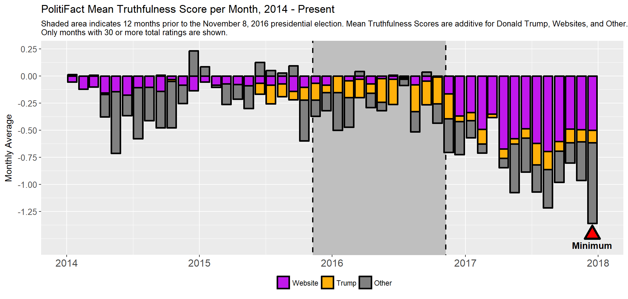
3. Subject
# Topics#######

webpage <- read_html("http://www.politifact.com/subjects/")

#This gets the list of topics that PolitiFact's ratings pertain to
#I get the attributes, or the hyperlink from each of those topics to be able to scrape them
topics <- vector("list", length = 152)
for(i in seq_along(1:152)) {
  topics[[i]] <- html_attrs(
      html_nodes(webpage, ".az-list__item a"))[[i]][[1]]
}

combined_topics <- as_tibble(do.call("rbind", topics)) #Hyperlink to each topic

combined_topic_names <- as_tibble(      #Topic Name (Human-speak) for merging later
  html_text(
    html_nodes(webpage, ".az-list__item a")))

scorecard <- vector("list", length(topics))
count <- vector("list", length(topics))

for(i in seq_along(topics)) {
  webpage <- read_html(str_c("http://www.politifact.com",
                             combined_topics[[1]][[i]]))

  topics_scrape <- function(x) {
    as_tibble(
      html_text(
        html_nodes(webpage, x)))
  }

  scorecard[[i]] <- topics_scrape('.chartlist__label :nth-child(1)') %>%
    add_column(combined_topic_names$value[[i]]) #Adding the topic column
  colnames(scorecard[[i]]) <- c("scorecard", "topic") #Changing the column name to be able to bind

  count[[i]] <- topics_scrape('.chartlist__count') %>%
    add_column(combined_topic_names$value[[i]])
  colnames(count[[i]]) <- c("count", "topic")

  Sys.sleep(time = 2) #Sleepy sleepy
}

(combined_scorecard <- do.call("rbind", scorecard))
(combined_count <- do.call("rbind", count))

total_topics <- bind_cols(combined_scorecard, combined_count) %>%
  mutate(count = as.integer(
                    str_extract(count, "\\d{1,4}")),
         topic = str_replace_all(topic, "^\\s|\\s$", "")) %>%
  select(-topic1)

combined_topic_names <- combined_topic_names %>%
  mutate(str_replace_all(value, "^\\s|\\s$", ""))
total_topics <- total_topics %>%
mutate(scorecard = str_replace_all(scorecard, c("Half True" = "Half-True", "Pants on Fire$" = "Pants on Fire!")))
total_topic_ratings <- left_join(total_topics, values, by = c("scorecard" = "rating")) %>%
mutate(Score = value * count) %>%
group_by(topic)
total_topic_summary <- total_topic_ratings %>%
summarise(total_ratings = sum(count),
total_score = sum(Score)) %>%
mutate(Avg_Score = total_score / total_ratings) %>%
mutate(Pos_Neg = ifelse(Avg_Score >= 0, "Positive", "Negative"))
table_of_topics <- total_topic_summary %>%
filter(rank(desc(total_ratings)) < 11) %>%
arrange(desc(total_ratings)) %>%
mutate(`Mean Truthfulness Score` = round(Avg_Score, 3),
`Total Ratings` = comma_format()(total_ratings)) %>%
rename(Subject = topic) %>%
mutate(Rank = 1:10) %>%
select(Rank, Subject, `Total Ratings`, `Mean Truthfulness Score`) PolitiFact groups together many of the statements it rates by the subject that statement addresses (e.g. Abortion, Patriotism, Obama Birth Certificate, etc.) here. PolitiFact also notes the frequency with which it assigns its six ratings (i.e. True, Mostly True, Half-True, Mostly False, False, and Pants on Fire!) to statements in each subject. Currently there are 149 different subjects. The most frequently discussed subjects and their Mean Truthfulness Scores are below:
kable(table_of_topics, align = c("c", "l", "r", "r"),
caption = "Most Discussed Subjects in PolitiFact Ratings")| Rank | Subject | Total Ratings | Mean Truthfulness Score |
|---|---|---|---|
| 1 | Health Care | 1,580 | -0.582 |
| 2 | Economy | 1,508 | -0.067 |
| 3 | Taxes | 1,340 | -0.278 |
| 4 | Education | 996 | -0.102 |
| 5 | Jobs | 962 | -0.166 |
| 6 | Federal Budget | 958 | -0.170 |
| 7 | State Budget | 920 | -0.216 |
| 8 | Candidate Biography | 830 | -0.488 |
| 9 | Elections | 826 | -0.317 |
| 10 | Immigration | 747 | -0.503 |
Looking at the most truthfully discussed and most falsely discussed subjects, it comes as no surprise that topics such as “Fake news” and Obama’s Birth Certificate have very negative Mean Truthfulness Scores. I leave it to others to ponder why topics such as “Population”, “Redistricting”, and “Gambling” are more truthfully discussed.[^3] I believe part of it has to do with uneven statement sampling.
top_10 <- total_topic_summary %>%
  filter(total_ratings >= 30) %>%
  filter(rank(desc(Avg_Score)) < 11) %>%
  arrange(desc(Avg_Score))

bottom_10 <- total_topic_summary %>%
  filter(total_ratings >= 30) %>%
  filter(rank(Avg_Score) < 11) %>%
  arrange(Avg_Score)

both_10s <- bind_rows(top_10, bottom_10) %>%
  mutate(topic = as_factor(topic),
         topic = fct_reorder(topic, Avg_Score))
ggplot(both_10s, aes(x = topic, y = Avg_Score, fill = Pos_Neg)) +
geom_col(size = 1, color = "black") +
geom_vline(xintercept = 10.5, size = 1.5, linetype = "twodash") +
coord_flip() +
scale_fill_manual(values = c("Positive" = "#71BF44", "Negative" = "#E40602")) +
theme(legend.position = "none",
axis.text = element_text(size = 12),
axis.title = element_text(size = 12)) +
labs(x = "", y = "Mean Truthfulness Score",
title = "Top 10 Most Truthfully Discussed and Most Falsely Discussed Truth-O-Meter Subjects",
subtitle = "Only subjects with at least 30 rated statements are included.") +
scale_y_continuous(limits = c(-3, 0.5), breaks = c(-3:0, 0.5))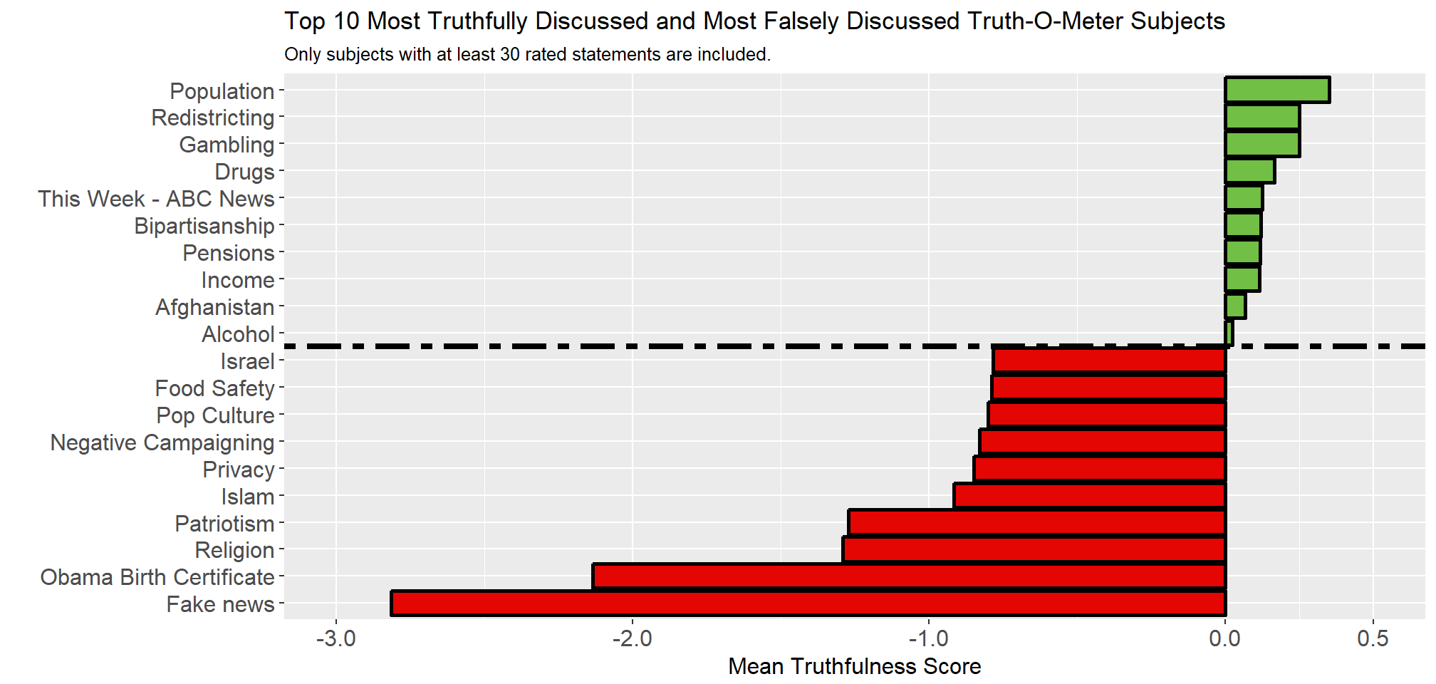
4. Individuals
# Senators and Representatives: ###############
# This includes Congressional Sessions 109-115 (i.e. 2007-2008 to 2017-2018) in order to capture when PolitiFact
# started on their ratings
individual <- vector("list", 10)
expanded_info <- vector("list", 10)

for(i in seq_along(1:10)) {
webpage <- read_html(str_c("https://www.congress.gov/members?q=%7B%22congress%22%3A%5B%22110%22%2C%22111%22%2C%22112%22%2C%22113%22%2C%22114%22%2C%22115%22%5D%7D",
                 "&page=", i))

politifact_scrape <- function(x) {
  as_tibble(
    html_text(
      html_nodes(webpage, x)))
}

individual[[i]] <- politifact_scrape(".result-heading a")
expanded_info[[i]] <- politifact_scrape(".expanded")

Sys.sleep(time = 2)
}

combined_rep_names <- unique(do.call("rbind", individual)) #It was duplicating the names for some reason
combined_expanded_info <- do.call("rbind", expanded_info)

congress <- bind_cols(combined_rep_names, combined_expanded_info)
congress <- congress %>%
  rename(Individual = value, Information = value1) %>%
  mutate(Individual = str_replace(Individual, "[[:alpha:]]*\\s", ""),
         State = str_extract(Information, "(?<=State:[[:space:]]{1,100})[[:alpha:]]+\\s*[[:alpha:]]+(?=\\r)"),
         Party = str_extract(Information, "(?<=Party:[[:space:]]{1,100})[[:alpha:]]+\\s*[[:alpha:]]+(?=\\r)"),
         Served = str_extract(Information, "(?<=Served:[[:space:]]{1,100})[[:alpha:]]+:.*(?=[[:space:]])")) %>% #I actually don't use this info, because it was too messy in the real-world to be suitable in my opinion for analysis, but I'm really proud that I was able to get a regex to find it. Messy in that many senators and reps and governors held multiple of each position, and they quit and swapped at frequently non-coinciding dates.
  separate(col = Individual, into = c("Last Name", "First Name"), sep = "\\,\\s") %>%
  select(-Information) %>%
  unite(col = Individual, `First Name`, `Last Name`, sep = " ", remove = TRUE)
current_governors <- read_csv("D:/Everything/R/Politifact Investigation/tabula-Current Governors List.csv", skip = 3, col_names = FALSE) #This came from
#running Tabula on this pdf https://www.nga.org/files/live/sites/NGA/files/pdf/directories/GovernorsList.pdf
not_states <- tibble(x = c("American Samoa", "Guam", "Northern Mariana Is.", "Puerto Rico", "Virgin Islands")) #Taxation without Representation
current_governors <- current_governors %>%
rename(State = X1, Governor = X2, Term = X4) %>%
separate(col = Governor, into = c("Governor", "Party"), sep = "\\(") %>%
mutate(Party = str_replace_all(Party, "[[:punct:]]", ""),
Term = str_replace_all(Term, "(?<=-\\d{2}).*$", ""),
Status = "Current") %>%
filter(!State %in% not_states$x) %>%
select(State, Governor, Party, Term, Status)
former_govs <- read_csv("D:/Everything/R/Politifact Investigation/Former Governors Copied.csv") #I had to copy this manually from
# https://en.wikipedia.org/wiki/List_of_living_former_United_States_Governors into a csv
former_govs <- former_govs %>%
filter(!is.na(Governor),
Governor != "Governor") %>%
rename(Term = `Term(s)`) %>%
mutate(Party = str_replace_all(Party, "\\w*,", ""),
Party = str_extract(Party, "Democratic|Republican"), # Only taking their later political stance
Status = "Former") %>%
select(State, Governor, Party, Term, Status)
governors <- as_tibble(bind_rows(current_governors, former_govs))#2016 presidential candidates
webpage <- read_html("https://www.nytimes.com/interactive/2016/us/elections/2016-presidential-candidates.html?_r=0")
politifact_scrape <- function(x) {
as_tibble(
html_text(
html_nodes(webpage, x)))
}
Prez_Cand_2016 <- politifact_scrape(".g-profile .g-name")
Prez_Cand_2016 <- Prez_Cand_2016 %>%
separate(value, into = c("Candidate", "Party"), sep = -2) %>%
mutate(Party = str_replace_all(Party, c("d$" = "Democratic", "r$" = "Republican")),
Affiliation = "Presidential Candidate",
Time = 2016)
#2012
Prez_Cand_2012 <- tibble(Candidate = c("Mitt Romney", "Rick Santorum", "Ron Paul", "Newt Gingrich", "Herman Cain"),
Party = rep("Republican", 5)) %>% #from https://en.wikipedia.org/wiki/Republican_Party_presidential_primaries,_2012
mutate(Affiliation = "Presidential Candidate",
Time = 2012)
#2008
webpage <- read_html("https://www.nytimes.com/elections/2008/primaries/candidates/index.html")
Prez_Cand_2008_D <- politifact_scrape('#not_running+ .o8column .o8name a')
Prez_Cand_2008_D <- Prez_Cand_2008_D %>%
mutate(Party = "Democratic")
Prez_Cand_2008_R <- politifact_scrape('.o8column+ .o8column .o8out .o8name a')
Prez_Cand_2008_R <- Prez_Cand_2008_R %>%
mutate(Party = "Republican")
Prez_Cand_2008 <- bind_rows(Prez_Cand_2008_D, Prez_Cand_2008_R) %>%
rename(Candidate = value) %>%
mutate(Affiliation = "Presidential Candidate",
Time = 2008)#Combining all the candidates, governors and congress together separately, and then together together
presidential_candidates <- bind_rows(Prez_Cand_2008, Prez_Cand_2012, Prez_Cand_2016) %>%
rename(Person = Candidate) %>%
mutate(Time = as.character(Time))
governors <- governors %>%
rename(Person = Governor,
Time = Term,
Affiliation = Status) %>%
mutate(Party = str_replace_all(Party, c("R$" = "Republican", "D$" = "Democratic",
"I$" = "Independent")),
Affiliation = str_c(Affiliation, "Governor", sep = " ")) %>%
unite(col = Affiliation, Affiliation, State, sep = " ", remove = TRUE) %>%
select(Person, Party, Affiliation, Time)
congress <- congress %>%
rename(Person = Individual, Time = Served, Affiliation = State) %>%
mutate(Affiliation = str_c(Affiliation, " Congress"))
#Yeah this required a lot of manual adjusting and some manual adding
individuals <- bind_rows(governors, congress, presidential_candidates) %>%
mutate(Person = str_replace_all(Person, "^ | $", ""),
Person = str_replace_all(Person, c("Hillary Rodham Clinton" = "Hillary Clinton",
"Paul D. Ryan" = "Paul Ryan",
"Joseph R. Biden" = "Joe Biden",
"John A. Boehner" = "John Boehner",
"Rudolph W. Giuliani" = "Rudy Giuliani",
" \\w\\. " = " ",
"Russell Feingold" = "Russ Feingold",
"Jon Huntsman, Jr." = "Jon Huntsman",
"James Moran" = "Jim Moran",
"James Renacci" = "Jim Renacci",
"Christopher Dodd" = "Chris Dodd",
"J. Randy Forbes" = "Randy Forbes",
".*Bobby.* Scott" = "Bobby Scott",
".*Hank.* Johnson" = "Hank Johnson",
"George Bush" = "George W. Bush",
"Joseph Lieberman" = "Joe Lieberman"))) %>%
add_row(Person = "Donald Trump", Party = "Republican", Affiliation = "President", Time = "January 20, 2017") %>%
add_row(Person = "Al Gore", Party = "Democratic", Affiliation = "Vice-President", Time = "1993 - 2000") %>%
add_row(Person = "Dick Cheney", Party = "Republican", Affiliation = "Vice President", Time = "2001 - 2008") %>%
filter(!duplicated(Person)) #Remove the duplicate entries
people_speakers <- politifact %>%
filter(website == FALSE, #Not a website
str_detect(name, #Not including any of these elements, though it really doesn't matter
regex("\\d| for |Democrat|Republican|National|Committee|Party|ACLU|Crossroads|Activist| in | our |USA|U.S.|Prop| on |Freedom|PAC", ignore_case = TRUE)) == FALSE) %>%
mutate(name = str_replace_all(name, " ", " ")) %>%
group_by(name, rating) %>%
summarise(n = n())
verified_people_speakers <- inner_join(people_speakers, individuals, by = c("name" = "Person")) %>%
filter(Party %in% c("Democratic", "Republican")) %>%
distinct(name, rating, n, Party)
duplicates_check <- verified_people_speakers %>% #Check for politicians having changed their party
group_by(name, Party) %>%
distinct(Party)
duplicates_check$name[duplicated(duplicates_check$name) == TRUE]
old_politicians <- verified_people_speakers %>%
filter(name == "Charlie Crist", Party == "Republican") #Charlie Crist changed from Republican to Democrat, so his statements were duplicated. I will identify him as Democrat and remove the duplicate from when he was a republican
#Verified important politicians - this is the important one
verified_people_speakers <- anti_join(verified_people_speakers, old_politicians)
#Who wasn't joined
not_joined <- anti_join(people_speakers %>% group_by(name) %>% summarise(total_ratings = sum(n)),
individuals, by = c("name" = "Person")) #Note that this includes pundits, organizations, and state-level politicians
#Who else was a major politician that I haven't been able to match up? Many of them probably don't have statement ratings.
left_to_join <- anti_join(individuals,
people_speakers %>% group_by(name) %>% summarise(total_ratings = sum(n)), by = c("Person" = "name")) number_of_politicians <- verified_people_speakers %>%
group_by(Party) %>%
distinct(name) %>%
summarise(`Number of Politicians Rated` = n())
party_statements <- verified_people_speakers %>%
group_by(Party, rating) %>%
summarise(Subtotal_Ratings = sum(n)) %>%
ungroup() %>%
group_by(Party) %>%
mutate(`Total Ratings` = comma_format()(sum(Subtotal_Ratings))) %>%
spread(rating, Subtotal_Ratings) %>%
select(-`Total Ratings`, everything(), `Total Ratings`)
nominal_party_statements <- left_join(party_statements, number_of_politicians, by = c("Party" = "Party")) %>%
select(Party, `Number of Politicians Rated`, everything())
number_party_statements <- verified_people_speakers %>%
group_by(Party, rating) %>%
summarise(Subtotal_Ratings = sum(n)) %>%
ungroup() %>%
group_by(Party) %>%
mutate(Total_Ratings = sum(Subtotal_Ratings)) %>%
spread(rating, Subtotal_Ratings) %>%
select(-Total_Ratings, everything(), Total_Ratings)And finally, the last part of my analysis looks at various U.S. elected politicians’ individual records with the Truth-O-Meter. My intent has been to capture the most important U.S. politicians, whom I have defined to include current and recently former Presidents, Vice-Presidents, Presidential Candidates, Senators, Representatives, and Governors. [^4] In total, I will focus on the 467 Democratic and Republican U.S. politicians from these groups who have made statements that PolitiFact has rated.
Interestingly, PolitiFact has rated statements by 19.2% more Republican politicians than Democratic ones (254 vs. 213) but it has rated 62.7% more statements by Republican politicians than statements by Democratic ones (4,085 vs. 2,511). See the table below:
kable(nominal_party_statements, align = c("l", "r", "r", "r", "r", "r", "r", "r", "r"),
caption = "Number of Statements by Major U.S. Politicians by Party")| Party | Number of Politicians Rated | Pants on Fire! | False | Mostly False | Half-True | Mostly True | True | Total Ratings |
|---|---|---|---|---|---|---|---|---|
| Democratic | 213 | 69 | 308 | 331 | 596 | 682 | 525 | 2,511 |
| Republican | 254 | 306 | 890 | 802 | 822 | 693 | 572 | 4,085 |
peoples_scores <- left_join(verified_people_speakers, values, by = c("rating" = "rating")) %>%
  mutate(sub_score = n * value) %>%
  ungroup() %>%
  group_by(name, Party) %>%
  summarise(total_ratings = sum(n),
         sum = sum(sub_score),
         score = sum / total_ratings) %>%
  filter(total_ratings > 30) #There really aren't that many politicians with at least 30 statements - perhaps I should lower that but I kept it for consistency's sake with the earlier graph of PolitiFact's statements by month

top_5_peoples_scores <- peoples_scores %>%
  group_by(Party) %>%
  filter(rank(desc(score)) < 6) %>% #This is an annoying way of getting the top or bottom 5
  arrange(desc(score)) %>%
  filter(score >= 0)

bottom_5_peoples_scores <- peoples_scores %>%
  group_by(Party) %>%
  filter(rank(score) < 6) %>%
  arrange(score) %>%
  filter(score <= 0)

top_bot_5_both <- bind_rows(top_5_peoples_scores, bottom_5_peoples_scores) %>%
  ungroup() %>%
  mutate(name = as_factor(name),
         name = fct_reorder(name, score),
         color = ifelse(Party == "Democratic", "#1A80C4", "#CC3D3D"))


dems_repubs_function <- function(number, party) {
  the_tibble <- top_bot_5_both %>%
    top_n(number, score) %>%
    filter(Party == party)

  str_c(the_tibble$name, collapse = ", ") %>%
    str_replace_all(", (?=\\w+\\s\\w+$)", ", and ") #Another cute little Regex I'm proud of that converts it all to correct English.
}
top_dems <- dems_repubs_function(10, "Democratic")
bottom_dems <- dems_repubs_function(-10, "Democratic")
top_repubs <- dems_repubs_function(10, "Republican")
bottom_repubs <- dems_repubs_function(-10, "Republican")
Next, I will look at which politicians have the highest Mean Truthfulness score by party. The five Democratic politicians with the highest Truthfulness Score are Sherrod Brown, Tim Kaine, Hillary Clinton, Bill Clinton, and Barack Obama while the five Democrats with the lowest Truthfulness Score are Terry McAuliffe, Nancy Pelosi, Debbie Wasserman Schultz, Tammy Baldwin, and Joe Biden. The five Republican politicians with the highest Truthfulness Score are Rob Portman, Nathan Deal, John Kasich, Jeb Bush, and Rand Paul while the five Republicans with the lowest truthfulness score are Michele Bachmann, Donald Trump, Ted Cruz, Newt Gingrich, and Rick Santorum. The five least truthful Democrats all have a higher Mean Truthfulness Score than the five least truthful Republicans.
colors <- top_bot_5_both$color[order(top_bot_5_both$name)] #Had to post on stackoverflow to figure this one out

ggplot(top_bot_5_both, aes(x = name, y = score, fill = Party)) +
  geom_col(size = 1, color = "black") +
  coord_flip() +
  geom_vline(xintercept = 10.5, size = 1.5, linetype = "twodash") +
  scale_fill_manual(values = c("Democratic" = "#1A80C4", "Republican" = "#CC3D3D")) +
  labs(y = "Mean Truthfulness Score", x = "",
       title = "Top 5 Individual Highest and Lowest Mean Truthfulness Scores by Party",
       subtitle = "Only major U.S. politicians with at least 30 rated statements are included") +
  theme(axis.text = element_text(size = 12),
        axis.text.y = element_text(color = colors),
        axis.title = element_text(size = 14),
        legend.position = "bottom",
        legend.title = element_blank())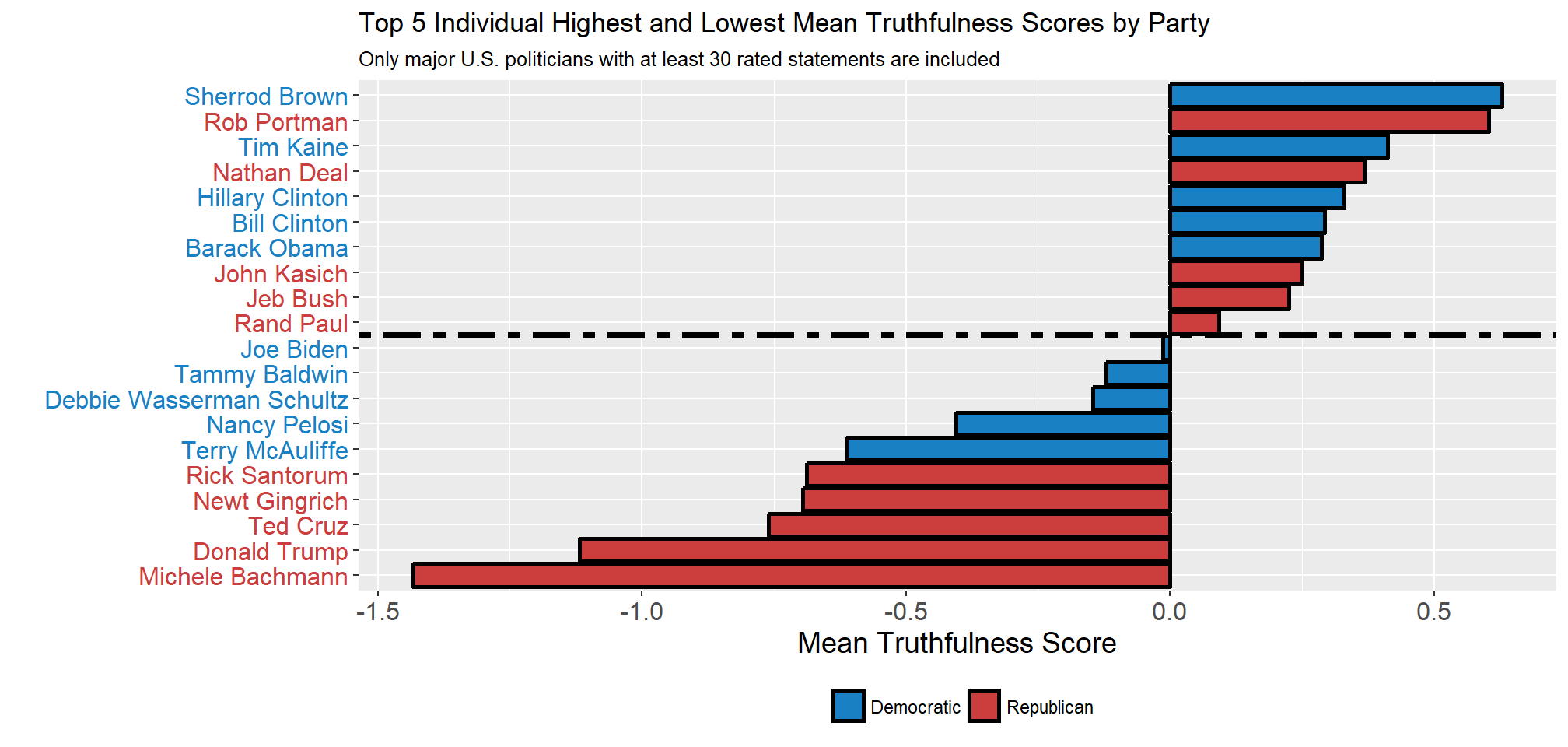
#For the maxim below
Those_Who_Lie <- verified_people_speakers %>%
  filter(name %in% peoples_scores$name) %>%
  group_by(name) %>%
  filter(rating == "Pants on Fire!" | rating == "False")

Those_Who_Dont <- peoples_scores %>%
  filter(!name %in% Those_Who_Lie$name)
Currently, there are 0 major U.S. Politicians who have not made a False or Pants on Fire! statement, among those with 30 or more statements rated by PolitiFact. The adage that “All politicians lie” seems to be accurate, but it should be followed up with “but some lie a lot more than others.”
4.1 Overall Party Mean Truthfulness Score
politifact <- politifact %>%
  mutate(name = str_replace_all(name, "  ", " ")) %>%
  mutate(rating = fct_drop(rating))

politifact <- left_join(politifact, values, by = "rating")

party_statistical_test <- inner_join(politifact,
                                      verified_people_speakers %>%
                                        filter(!duplicated(name)) %>%
                                        select(name, Party),
                                      by = c("name" = "name"))

democrats <- party_statistical_test %>%
  filter(Party == "Democratic")
republicans <- party_statistical_test %>%
  filter(Party == "Republican")
The final part of my analysis includes grouping all of the major U.S. politicians who have received ratings from PolitiFact by party. This may be an accurate reflection of which party is more “truthful” or it may reflect selection-bias by me or by PolitiFact. Nonetheless, after performing a z-test on statements by major U.S. politicians from the Democratic and Republican party, I can say with greater than 99% confidence that the Mean Truthfulness Score for statements made by major U.S. Democratic politicians is statistically higher than that for major U.S. Republican politicians. [^5]
party_politicians <- verified_people_speakers %>%
  group_by(Party, rating) %>%
  summarise(`Total Statements` = sum(n))

party_politicians <- left_join(party_politicians, values, by = c("rating" = "rating")) %>%
  mutate(score = value * `Total Statements`) %>%
  group_by(Party) %>%
  summarise(Total_Statements = sum(`Total Statements`),
            Score = sum(score)) %>%
  mutate(Final_Ratings = Score / Total_Statements)

added_row <- tibble(Party = "Average Major U.S. Politician",
                    Total_Statements = sum(party_politicians$Total_Statements),
                    Score = sum(party_politicians$Score),
                    Final_Ratings = Score / Total_Statements)

party_politicians <- party_politicians %>%
  bind_rows(added_row) %>%
  mutate(Party = as_factor(Party),
         Party = fct_relevel(Party, "Average Major U.S. Politician", after = 2))
ggplot(party_politicians, aes(x = Party, y = Final_Ratings, fill = Party,
label = round(Final_Ratings, 3))) +
geom_col(size = 1, color = "black") +
scale_fill_manual(values = c("Democratic" = "#1A80C4", "Republican" = "#CC3D3D", "Average Major U.S. Politician" = "#735F81"), guide = "none") +
labs(x = "", y = "",
title = "Mean Truthfulness Score for Major Politicians' Statements by Party",
subtitle = str_c("Includes ",
comma_format()(sum(party_politicians %>%
filter(Party == c("Democratic", "Republican")) %>%
select(Total_Statements))),
" statements rated by PolitiFact from ",
nrow(verified_people_speakers %>%
group_by(name) %>%
summarise(n = n())),
" current and recent major U.S. politicians, including:\nPresidents, Vice-Presidents, Presidential Candidates, Senators, Representatives, and Governors.")) +
geom_hline(yintercept = 0, size = 1.5, linetype = "twodash") +
geom_vline(xintercept = 2.5, size = 1.5, linetype = "solid") +
theme(axis.text = element_text(size = 12),
axis.text.x = element_text(color = c("#1A80C4", "#CC3D3D", "#735F81"), face = "bold"),
panel.grid.major.x = element_blank()) +
geom_label()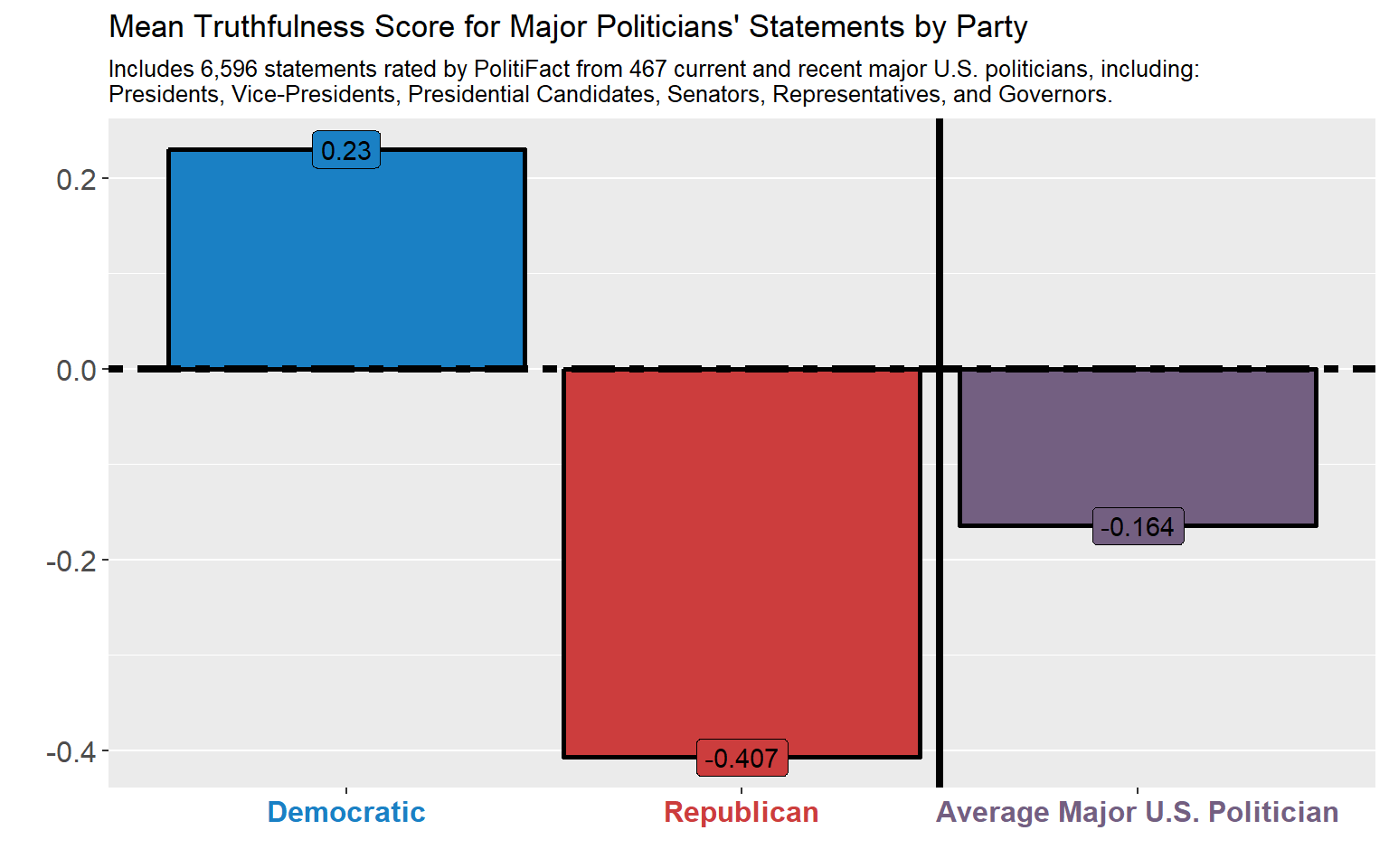
5. Final Words
This project is simply an effort to improve my data wrangling and analysis skills as well to create a personal and demonstrable product of my abilities. While I have no connection to PolitiFact, I deeply appreciate the work they do and I encourage others to do the same. I apologize for using up their server space while scraping their site, but hopefully any exposure of their work and financial contributions from myself and others can more than repay that.
For information on joining PolitiFact, see here.
If you have any suggestions about ideas to extend this analysis, please share them. You are free to share this github site (attributing me as the author) or to use any of the R code I have written for your own private, non-commercial use. Simply put, please respect the time and effort I put into this project.
Footnotes
[^1] Not until I had done a lot data wrangling did I realize that PolitiFact seems to be missing from its site any ratings issued in November 2008. While it has ratings through October 31, 2008 and beginning again on December 1, 2008, there are no ratings at all for November 2008. Visit this page and nearby ones to verify (http://www.politifact.com/truth-o-meter/statements/?page=669)
[^2] It appears that PolitiFact’s efforts to fact-check claims appearing on Facebook do not appear in its Truth-O-Meter ratings, which puts them beyond the scope of my analysis. When I discuss PolitiFact’s ratings of statements made by websites, I only analyze those that appear in PolitiFact’s Truth-O-Meter ratings.
[^3] Not all subjects listed on PolitiFact’s subjects page are actual issues. While subjects such as Abortion and Islam capture statements that refer to Abortion or Islam, the subject “This Week - ABC News” captures statements instead made by politicians and pundits while actually on that television show.
[^4] PolitiFact has rated statements by 3,666 different entities. In my analysis of statements by major politicians by their political party, I used the following lists:
- U.S. Senators and Representatives from the 109th to the 115th Congressional Sessions, available here. I included all of the sessions that have overlapped with PolitiFact’s existence, which began in 2007.
- Current U.S. State Governors, available here
- Currently living former U.S. State Governors, available here
- 2008, 2012, and 2016 presidential candidates
- The eight Presidents and Vice-Presidents from 1993 to Present (PolitiFact has not yet rated any statements by presidents prior to Bill Clinton).
When I refer to ‘Democrats’ and ‘Republicans’ in my analysis, I am referring to politicians from the above lists who I have been successfully able to match to individuals who have had statements rated by PolitiFact. Because the matching process is difficult, I cannot guarantee that every individual who falls into the following categories has been accounted for but this should include enough politicians to make my conclusions and analysis valid. I furthermore sought to ensure that every valid U.S. politician who has had at least 10 statements rated by PolitiFact was included. The political party designation used comes from the above mentioned sources.
The remaining entities whose individual records I have intentionally not chosen to analyze include:
- Organizations, civic initiatives, PACs, campaigns, party committees and the like
- Websites
- Pundits such as Rush Limbaugh, Sean Hannity, Rachel Maddow, etc.
- And Politicians whose only positions thus far are:
- At the state level
- In a non-elected appointment (i.e. to the cabinet level, ambassadorship, or the Supreme Court)
- Unsuccessful campaigns for a political seat (other than U.S. president)
- Not-yet assumed office (i.e. Governor-elect, Senator-elect, etc., but I do include Presidents-elect)
- Or not clearly associated with either the Democratic or Republican parties (e.g. I have excluded Gary Johnson, Ralph Nader, and Jesse Ventura, but not Bernie Sanders or Joe Lieberman).
- At the state level
Keep in mind that many politicians who did fit my criteria may at some point have held a position on the above list.
final_test <- z.test(x = democrats$value, y = republicans$value, alternative = "two.sided",
                     sigma.x = sd(democrats$value), sigma.y = sd(republicans$value), conf.level = 0.99)
[^5] A z-test is used when the population variance and standard-deviation are known. Because I am considering the population only to be the statements that PolitiFact has rated (rather than all statements all politicians have made), I believe a z-test is more appropriate than a t-test. For Democrats, the standard deviation of their Mean Truthfulness Score is 1.388 and for Republicans it is 1.519 (all numbers in this footnote are rounded to three digits). In the z-test, the null hypothesis is that the true difference between the Mean Truthfulness Score of Democrats and Republicans is equal to zero; currently the difference between those means is 0.637. With 99 percent confidence, the true difference between these means is estimated to be between 0.543 and 0.731.
save.image("D:/Everything/R/Politifact Investigation/Final_Final_Workspace.Rdata") #Save the workspace so I can use it in the 'Analysis' page without having to re-run all this code